Selecting the Right XGBoost Loss Function in SageMaker

XGBoost is an open source software library to apply the gradient boosting framework to supervised learning (SL) tasks. Because of its effectiveness, speed, and robustness in solving a wide variety of SL problems, a current saying is that the best type of model for your SL problem is either a deep learning algorithm or XGBoost. As a result of its well-deserved popularity, XGBoost is available as a built-in model in Amazon SageMaker, a cloud machine learning platform.
With minimal knowledge of the XGBoost framework, any data scientist can easily plug in their dataset and produce an XGBoost model in SageMaker. Since SageMaker offers baysian hyperparameter tuning, which will retrain and select the best model across different hyperparameters, users can get away without fully understanding key inputs like max_depth and eta. However, there is often little consideration of the loss function (objective) to use when training XGBoost, even though it may be the most important human decision in the process. This article aims to provide more insight into how to select the right loss function when training XGBoost or other SL models for regression tasks.
Let's start by explaining gradient boosting. A helpful start is to understand what isn't gradient boosting -one example being the ensemble decision tree algorithm, random forest. Ensemble decision tree algorithms are those that aim to produce several ‘weak-learner' trees that when used in a network produce a ‘strong learner'. Let's say we have an ensemble of 100 trees, random forest conceptually produces each of these trees in parallel, using ‘bagging' to select a subset of observations and dimensions to use to produce each tree, then takes a weighted average of the predictions of all 100 trees to get the final prediction for a regression problem.
The key difference with XGBoost is that individual trees can't be produced in parallel, they must be produced in sequence. Specifically, each subsequent tree in an XGBoost model is used to predict the error of the preceding tree. By using an ensemble approach with both ‘bagging' (pulling different observations and dimensions out of a bag for each tree), and ‘boosting' (building trees in sequence), XGBoost framework is able to reduce model bias without overfitting. Furthermore, XGBoost and other tree-based models are robust to high-variance datasets with low-importance dimensions.
Now that we understand how XGBoost works from a high-level, let's return the loss function. Loss functions take in model predictions for a set of observations and tell you how far they were from actual outcomes. For regression problems, the focus of this discussion, the simplest loss function that comes to the human mind is mean absolute error – we subtract the predictions from the actual values (or vice versa), take the absolute value, then take an average across all observations. In other words, missing by 200 is twice as bad as missing by 100.
But the standard loss function used for most XGBoost use cases is ‘reg:squarederror', formerly called ‘reg:linear' in SageMaker. The only difference with squared error and absolute error, as the name indicates, is that errors for each observation are squared before being averaged. Because squaring has a compounding effect as the size of errors increases, mean squared error penalizes large misses proportionally more than mean absolute error does. Missing by 200 is now 4X as bad as missing by 100.
But why would mean squared error be the standard, unquestioned, loss function used to train XGBoost and other SL models when it's just not as simple or intuitively sound as mean absolute error?
The first distinction to understand is that of prediction and estimation loss.

Prediction loss is the loss incurred by the business, while estimation loss is how far the model is from the ‘ground truth' model. The right estimation loss function isn't always the one that minimizes prediction loss. As I'll show later, you can reduce prediction loss by choosing a different estimation loss function.
Given mean average error does well at quantifying the penalty of missing in many real world cases, why does mean squared error often win when estimating the best model parameters?
It all comes down to the practical assumption of model errors being normally distributed.

Let's assume that there are two components required to perfectly explain an outcome, Y. First, the signal that can be derived from model dimensions. In this case, let's assume a linear model with a single dimension and a bias term is sufficient (mX + b below). And second, a random variable, Z, that follows a normal distribution with independent variance.
The best estimation loss function in a sense is the one that when applied to a model maximizes the likelihood of having produced the observed data. In this case, it turns out to be MSE.
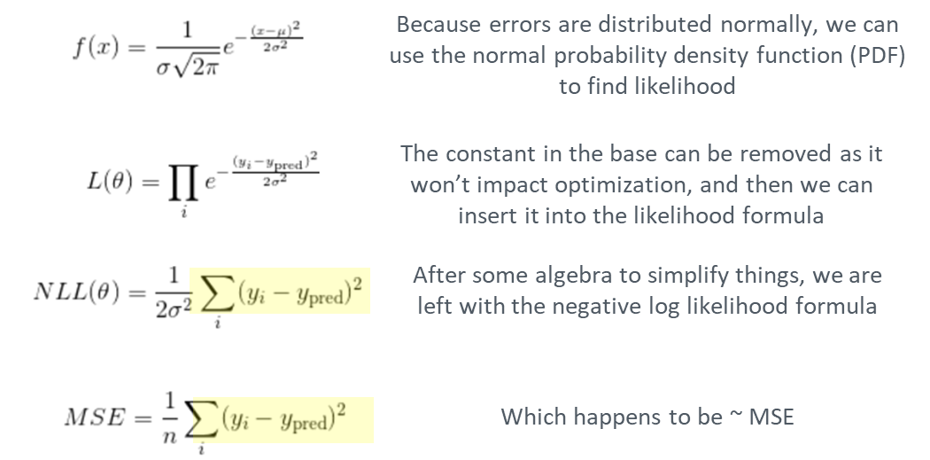
The appearance of the squaring can be traced back to the probability density function of the the normal distribution, which is essential to producing the bell shape.
But what if errors and specifically the random component, Z, are not distributed normally? Another common prediction error distribution observed in regression problems is the Laplace distribution.

When observing the probability density function of the Laplace distribution, the absolute error formula immediately sticks out. The lack of squaring results in an spike in the distribution about 0 on the X axis.

Furthermore, it turns out that mean absolute error is the loss function that maximizes likelihood of observing data when model errors follow the Laplace distribution.
Normal and Laplace distributions are only a couple of the error distributions that can be observed in regression tasks, however. For problems with count-based data, errors may follow a Poisson distribution. So in other cases, additional research be needed to find the matching error distribution and associated loss function that will lead to the best parameter estimates.
Without going any further, we already have an improved algorithm to select the the right loss function for an XGBoost model.
- Produce an arbitrary model.
- Observe errors and whether they closely resemble a normal or Laplace distribution.
- If they do, select a loss function of mean squared or mean absolute error, respectively.
- If not, research and test alternative distributions that match observed errors and are common for similar problems. Then, find the loss function that will lead to the most likely parameter estimates.
As a business case for the application of this simple algorithm, I will share a real SL regression case I encountered.
- An XGBoost model with a mean squared error loss was trained leading to the following prediction error distribution.

- Prediction errors closely resembled the Laplace distribution.
- Mean average error should be used as the loss function.
The only issue is that XGBoost and deep learning algorithms, our go-tos to solve the laundry list of SL problems, require a smooth loss function to perform gradient descent (or comparable optimization algorithm). So we need to find a smooth loss function that closely resembles mean absolute error. The best option available in SageMaker is pseudo-huber; the huber distribution is shown below which closely resembles absolute error at a delta of 1.

So for my use case, what were the impacts of switching from a squared error loss function to pseudo-huber and mean absolute error for model training and hyperparameter tuning?

In the chart, you can see the mean absolute error (MAE) dropped by 30% when pseudo-huber loss was paired with MAE hyperparameter tuning. More interestingly, even if the most important objective to the business was root mean squared error (RMSE), using an estimation loss function of mean absolute error resulted in improved business outcomes.
Closing remarks
While XGBoost and comparable ensemble decision tree models are making it easy for data scientists to plug and play with their different datasets and achieve good model performance with minimal effort, there is a price to pay for surface level understanding. Selecting the right loss function is one simple example which I showed can lead to a 30%+ model improvement.
On a deeper level, Data Science is all about asking why, pursuing the important details to illuminate the answer, and discarding the ones that are accessory. It requires intuition, pursuing your curiosity, digging in further when surprised, and breaking down a problem from the big picture to the fine print. This article outlines my journey to understand why mean squared error is considered the standard loss function for XGBoost regression tasks. The result is a simple system to prescribe the best loss function for a variety of cases. I hope this article was of use to you as you progress on your own pursuit to understand why and use what you uncover to help tackle important business challenges.
Thanks for reading! If you liked this article, follow me to get notified of my new posts. Also, feel free to share any comments/suggestions.
